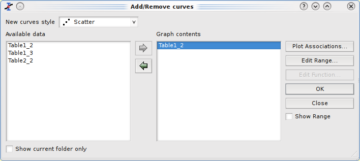
Opens the Add/Remove Curve dialog, allowing to easily add or remove curves from the active plot layer. This dialog can also be used to modify a curve which is already plotted by changing the columns which are used as X or Y values.

The left window shows the columns which are available for plotting in the different tables of the project, and the right window gives the list of the curves already plotted. In the case presented below, there are two tables in which the Add/Remove Curve dialog box allows to select columns. If you use this dialog box to add a column, the X column will be the one define as X in the corresponding table.

Figure 5.14. The Add/Remove Curve dialog box.

In this dialog box, if you select one curve of the plot in the right window, you can change the columns used for X and Y with the Plot Association button. In any case, you can't mix the X values of one table with the Y values of another one. If you wan't to do this, you have to copy the columns in the same table.

If the curve selected is a function, you can modify it. Refer to the Add Function command for more details on functions editing.

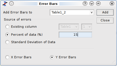
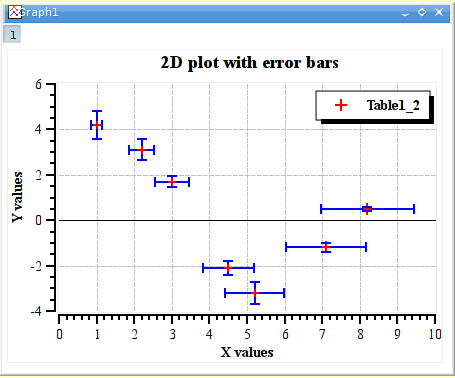
This command is used to plot X and/or Y error bars around the data points.

It must be taken care that the "add" button add the errors bars, and so do the "OK" button. Then, you should close the dialog with cancel if you have clicked on the "add" button.

Figure 5.15. The Add Error Bars dialog.

There are three ways to specify the size of the bar:

Figure 5.16. A plot with X and Y Error Bars.

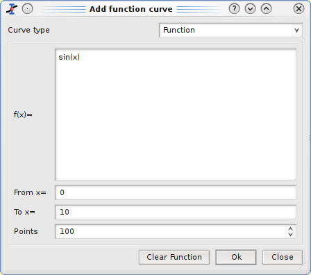
This dialog box is used to add a function curve to the active plot. The function can be built with the common operators: * + / - and ^ for the power. The intrinsic functions available are listed in the appendix.

The most common way to define a function is the classical cartesian coordinate definition y=f(x), this is the defaut option. The two following parameters allow to select the x range used for the plot, and the last one is used for the number of data points that are computed in the X-range.

Figure 5.17. The Add Function dialog box: cartesian coordinates.

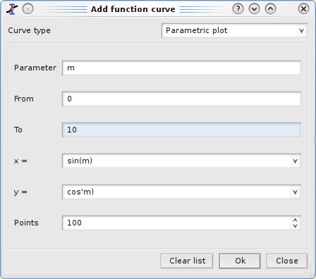
The functions can also be defined in a parametric definition: if t is the parameter, the (x,y) data points are computed by x=f(t) and y=g(t). The first parameter is the name of the parametric variable (here t) followed by the range, the definition of the two functions and the number of data points.

Figure 5.18. The Add Function dialog box: parametric coordinates.

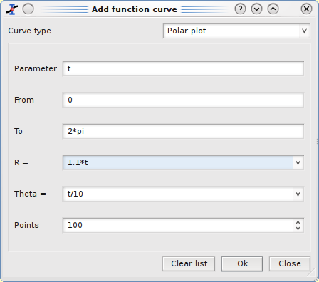
The last way is the polar definition of the function: if t is the parameter, the radius r and the angle theta are computed by r=f(t) and theta=g(t). Then the (x,y) data points are computed by x=r*cos(theta) and y=r*sin(theta).

The first parameter is the name of the parametric variable (here t) followed by the range, the definition of the two functions and the number of data points.The angle is defined in radians, and the constant value pi can be used: it is possible to use 3*pi to define the parameter range.

Figure 5.19. The Add Function dialog box: polar coordinates.

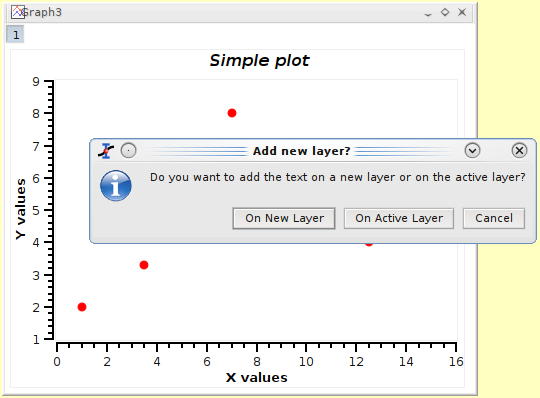
Opens a dialog allowing you to select whether the text is to be added to the active plot layer or on a new layer. The cursor changes to an edit text cursor. Next, you must click in the plot window to specify the position of the new text box. A text dialog will pop-up allowing you to type the new text to be displayed and all its properties (color, font, etc...)

If you choose the On new layer option, the text will be inserted as a new layer which has the size and the position of the text. You can then modify the size and position of this layer with the layer Geometry (see the Add Layer command for details). Beware that in this case, all text which is not in the layer will be clipped, therefore, you need to modify the layer to modify the position of the text. If you choose the On Active layer option, the text will be inserted in the selected layer, and its position can be modified directly with the mouse inside this layer.

Figure 5.20. The Add Text dialog box.

Changes the active layer operation mode to the drawing mode. You must click on the layer canvas in order to specify the starting point for the new arrow, and then click once more to specify its ending point. You can edit the new arrow using the Arrow dialog. You can swith back to the normal operating mode by clicking the "Pointer" icon in the Plot toolbar.

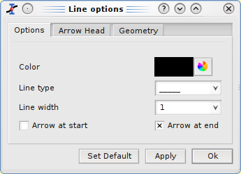
Then, a dialog allows to modify a line or an arrow which has been created. One can open it with a double click on an arrow or a line, or by selecting an arrow or a line and selecting Properties... with the right button of the mouse.

The first tab allows to change the color, the line type and the line width. This last parameter is set in pixels. It is possible to define a default style for all the new lines by pressing the Set Default button.

Figure 5.21. The Arrow options dialog: first tab

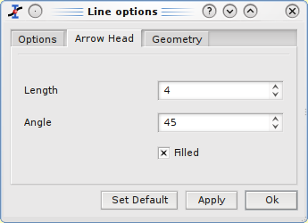
The Arrow head tab is used to modify the shape of the head of the arrow. The length is set in pixels and the angle is in degrees. It is also possible to define a default style for the arrow heads using the same Set Default button.

Figure 5.22. The Arrow options dialog: second tab

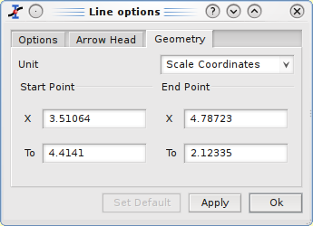
The Geometry tab allows to specify the start and end points of the line/arrow. The coordinates can be set as a function of the scales values displayed on the left axis (Y) and on the bottom axis (X) or in pixels, by choosing the desired method from the Unit pull-down list. The pixel coordinates are relative to the top-left corner of the layer which contains the line.

Figure 5.23. The Geometry dialog: third tab

Changes the active layer operation mode to the drawing mode. You must click on the layer canvas in order to specify the starting point for the new arrow, and then click once more to specify its ending point. You can edit the new arrow using the line dialog. You can swith back to the normal operating mode by clicking the "Pointer" icon in the Plot toolbar.

This command is used to add a special label in the current plot which contains the current date and time. The properties of this label can be customized like any other label that is added by the Add Text command.

A timestamp label is not modified if the plot is modified, saved, etc.

Opens a file dialog allowing you to select an image to be added to the active plot layer. Only a link to the image file will be saved into the project file and not the image itself. The new image is added to the left-top corner of the layer and can be moved by drag-and-drop.

Adds a new legend object to the active plot layer. You can have more than one legend on a plot. These legends can then be customized by double clicking on a given legend.

Restore the drawind parameters of the layout to its default values (as they are defined in the dialog box of the Arrange Layers command): margins between the layer and the window border of 5 pixels, layer centered in the window, etc.

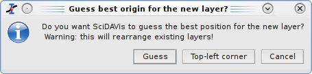
This dialog is opened when you want to add a new layer on the active plot. If you select Guess, SciDAVis will divide the window in two columns and put the new layer on the right. If you choose Top-Left Corner, SciDAVis will create a new layer with the maximum possible size over the existing layer, this layer contains an empty plot.

Figure 5.24. The Add Layer dialog box.

You can then modify the size and position of each layer by selecting it with the layer number buttons and selecting the Layer Geometry command from the context menu.

Deletes the active layer and prompts out a question dialog allowing you to choose whether the remaining layers should be automatically re-arranged or not.

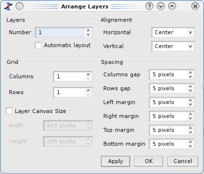
This dialog allows to modify the geometrical arrangement of the plots which are already present in the active window. You can also add new layers or remove existing ones.

Figure 5.25. The Arrange Layers dialog

The Arrange Layers dialog is used to modify the geometrical arrangement of the plots. You can specify the numbers of rows and columns which will define a table of plots. As pointed out above, you can also add or remove layers with this dialog, using the "Number of Layers" box.

With the default setting, SciDAVis computes the size of the layers from the size of the window. If you check the Layer Canvas Size, you can set the size of the layers and SciDAVis will modify the size of the window.

The two right zones allow to set the alignement of the layers in the window, and the margins between the layer borders and the window limits.

If you do some modifications on your plot, the alignment of the different axis may not be conserved. You can exec again the Arrange Layers to re-arrange your plot.