Table of Contents
The active items in the menus depend on the active window in the project. If the active window is a spreadsheet, then all the items linked to table functions are enabled and the others are automatically disabled.
These commands can also be done by clicking on the New Project icon from the File toolbar. In order to make this toolbar visible, use the Toolbars command from the View menu.
- File→ New →
- New→New Project (CTRL+N)
-
Creates a new SciDAVis project file. The project is the main container of SciDAVis, it can include tables, plots and notes. These objects can be organized in folders. If a project is open and saved, it will be closed. If a project is open is not saved, a dialog will be open to ask if the current project has to be saved. The new project will only contain an empty table.
These commands can also be done by clicking on the New Project icon from the File toolbar. In order to make this toolbar visible, use the Toolbars command from the View menu.
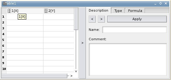
- New→New Table (CTRL+T)
-
Creates a new spreadsheet into the project. This empty table will have 30 rows and 2 columns. This number of rows and columns can be changed with the Dimensions command of the Table menu.
The properties of each column (format of numbers, width, etc) can be modified by the commands of the Table menu. See the table section for more details. There are then many different ways to insert data inside a table: they can be entered one by one, copied and pasted from another software like a spreadsheet, imported from a text file (see Import Ascii command), or filled with the result of a function as explained in the section Filling of a table with the values of a function.
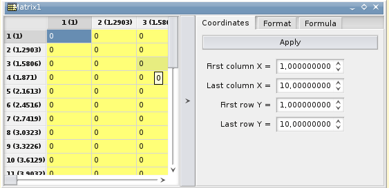
- New→New Matrix (CTRL+M)
-
Creates a new Matrix into the project. The empty matrix will have 32x32 cells, these dimensions can be changed by the Dimensions command of the Matrix menu. The default coordinates are ranging between 1 and 10 for x and y.
See the matrix section for more details.
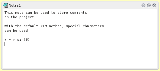
- New→New Note/Script (CTRL+ALT+N)
-
Creates a new note window in the project. A note is a simple text window which can be used to add comments to the current project.
This object is also used to store the scripts in python which can be used to perform complex operations with SciDAVis. See the note section and the python scripting sectionfor more details. It can also be used as a calculator.
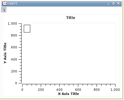
- New→New Graph (CTRL+G)
-
Creates a new empty 2D plot in the project. This default graph is just a framework in which you can add curves from the columns of a table with the Add/Remove Curve command or define a mathematical expression with the Add Function command (to access to these command, use the Graph menu or do a right click).
The graph will be created with the display parameters selected in the Preferences command (Edit menu).
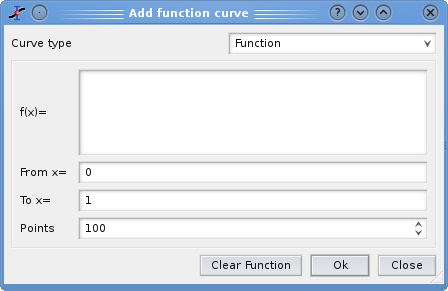
- New→New Function Plot (CTRL+F)
-
Opens a dialog allowing to create a plot by specifying an analytical function. See the 2D plot section of the tutorial for a general overview of this function.
This function can be defined in cartesian, parametric or polar coordinates, see the Add Function command for more details.
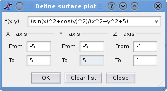
- New→New 3D Surface Plot (CTRL+ALT+Z)
-
Opens a dialog allowing to create a 3D plot by specifying an analytical function. See the 3D plot section of the tutorial for more detail on this function. The only available coordinate system is the cartesian one: z=f(x,y).
You can then enter the X, Y and Z scales.
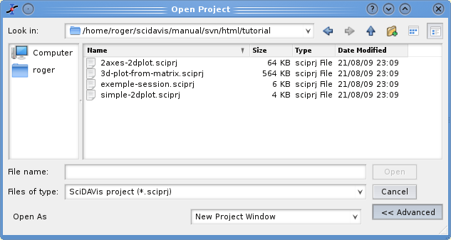
- File → Open (CTRL+O)
-
Opens an existing SciDAVis project file (default file extension .sciprj). If your project has been save in a compressed format, you must select the .sciprj.gz file format.
This command can also be used to open projects which have been built with the Qtiplot software (extension .qti) if the version used was below 0.9. By clicking on the Advanced button, an additional option appears which allows to insert a project in another as a new folder.
- File→ Recent Projects
Opens a list of the most recently used SciDAVis project files. You can open one of these files by selecting it from the list. If the file doesn't exist anymore an error message will pop-out and the file will be automatically deleted from the list.
- File→ Open image File (CTRL+I)
-
This command loads an image file in a SciDAVis project. This image can be resized and then inserted in another 2D plot. It is in this case similar to the Add Image command. This image can also be used to generate an intensity matrix (see the Import Image command).
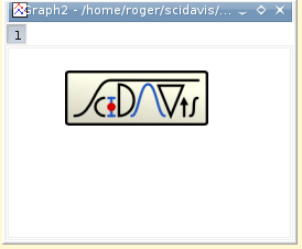
- File→ Import Image
-
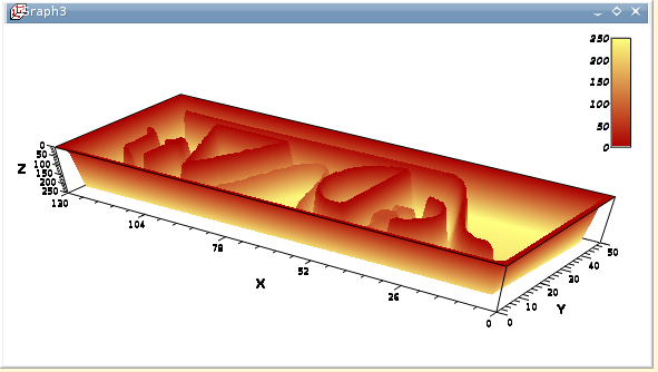
With this command, an image is loaded in the SciDAVis project and converted to an intensity matrix. For each pixel, an intensity between 0 and 255 is computed from the intensities of the three colors red, green and blue.
This example shows the 3D plot which has been drawn from the matrix obtained with the SciDAVis logo.
- File→ Save Project (CTRL+S)
-
Saves the actual project. If the project hasn't been saved yet ("untitled" project), a dialog will open, allowing to save the project to a specific location.In a project file all settings and all plots are stored in ASCII format.
If the project include large tables, it may be usefull to save the project in a compressed file format. The free zlib library is used to build files in gzip formats ( .sciprj.gz ).
- File→ Save Project As
Saves the actual project under a file name different from the current one.
- File → Open Template
-
Opens an existing template SciDAVis file. There are four kinds of templates with different extensions for file names.
Entity Extension Parameters saved 2D Plot .qpt window and layers geometries, fonts and colors for labels and legends, etc. Style for curves is not kept. 3D Plot .qst window and layers geometries, fonts and colors for labels and legends, etc Table .qtt number of row and columns Matrix .qmt number of row and columns You just have to add curves with the Add/Remove Curve command, but the style used to draw the curves is not kept in the template. See the the section called “Working with templates”.
- File → Save as Template
Save the active object as a SciDAVis template file. In the case of plot template (.qpt file), the graphical parameters of the plot, together with the text labels (axis, etc) are restored, but the style used to draw the curves and the scales are not saved.
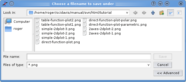
- File → Export Graph
-
The plot can be exported into several different image formats. You can define some parameters to customize your image file by checking the advanced options button. Depending on the chosen image format, the available options are not the same.
For tif, bmp, pbm, jpeg, xbm, pgm, ppm image formats, the quality of the image cannot be controlled, and these formats cannot handle transparency. Therefore, there is no need to check for advanced options.
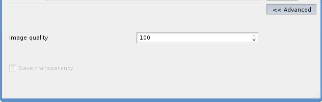
For jpeg and png, Image Quality parameter ranges between 0 and 100% and defines the compression ratio. The higher it is, the best the quality is but the larger the file is.
For png, tif and xpm, you can choose to use a transparent background.
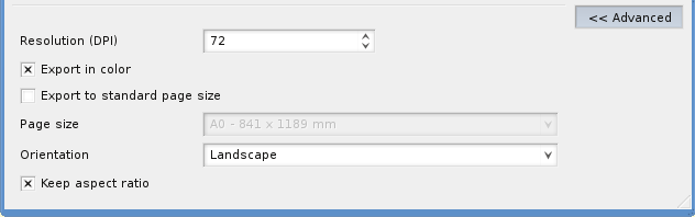
For eps, ps and pdf file format, the option dialog is different. The parameters availables are: the size of the paper which is used to draw the plot, and the orientation of the paper sheet. You can choose to keep or not the aspect ratio of the plot, in the last case it will be adapted to the sheet size and orientation.
In addition, you can define the resolution. The default value is 84. If you increase this parameter, the quality of the graphic elements will be better (but the overall size of the plot will be unchanged).
The last format which can be selected is the Scalable Vector Graphic format. With this format, the files can be modified in vector drawing software such as Sodipodi, Inkscape or OpenOffice Draw. You can therefore build more complex images from the pristine SciDAVis plot.
- Export Graph→Current (ALT+G)
Here you have the possibility to save the active plot under different image formats.
- Export Graph→All (ALT+X)
Here you have the possibility to save all plots of the project under different image formats. In this case, you must choose a directory for the differents plots. Then one file will be created for each plot, the filename being based on the title of the corresponding window.
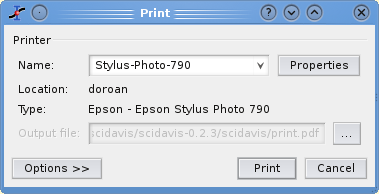
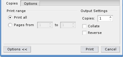
- File→ Print (CTRL+P)
-
Prints the active plot. A print dialog is opened where you can select the printer, etc.
.
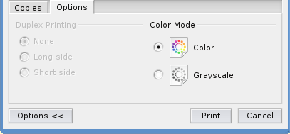
If your printer can handle duplex printing and/or color printing, your can select the corresponding options in the options tag of this dialog window.
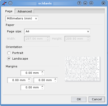
The properties button can be used to select the geometrics parameters of the printed output: paper size, margin, etc.
- File→ Print All Plots
Prints all plots of the projects. A print dialog is opened where you can select the printer, different paper sizes, etc.
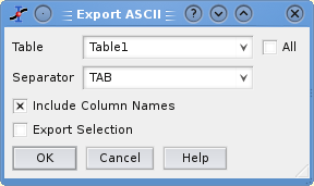
- File → Export Ascii
-
Opens a dialog box allowing to save the data from the active spreadsheet to an ASCII file. You can save one selected table, or all the tables of the project. You can then choose the field separator which will be used by SciDAVis. If you check Export Selection, only the selected cells will be saved; If not, the whole table will be exported, including the cells with no content.
When the options are selected, click on OK and a new dialog will be displayed to choose the file name. If you check the all checkbox, the dialog box will ask for a folder and each table will be save in a file named from the title of the table windows.
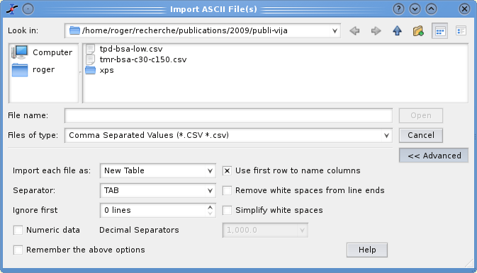
- File → Import Ascii
-
Imports one or more ASCII file into the project by creating a new spreadsheet storing the data from the file.
You can choose to put each data file in a separate table, or join all the data files in one table. There is no automatic analysis of the data. Therefore, by default, the data will be read as text. If you want to obtain directly numeric values, you can specify it in the numeric data check box. You must then indicate the format of the numbers. The other possibility is to read data as text and then to specify the type and format of the different columns with the properties dialog of the tables.
If you check the Remember the above options, the selected parameters will be used as default values. They will be used if you read an ascii file directly from the command line (see the Command line options section for more details.
- File → Quit (CTRL+Q)
Closes the application. You will be asked wether you want to save your last changes or not.