The commands which are available in this menu are not the same if a table or a plot is selected. For most analysis commands, you car refer to the tutorial in Chapter 3, Analysis of data and curves.
- Statistics on Columns
-
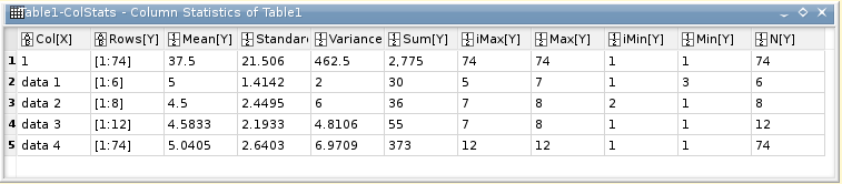
Creates a new table providing basic statistical information about the selected columns in the active table: average, variance, standard deviation, max value, etc...
You can select several columns in one table, one line will be created for each column. You can't select columns in different tables to obtain one single table of statistics.
- Statistics on Rows
-
Creates a new table providing basic statistical information about the selected rows in the active table: average, variance, standard deviation, max value, etc...
See the Statistics on Columns command command for more details.
- FFT
Computes a direct or inverse Fast Fourier Transform. See the the section called “Fast Fourier Transform” of the Chapter 3, Analysis of data and curves for more details.
- Correlate
Does a cross-correlation of the two columns which are selected. See the the section called “Correlation and autocorrelation” of the Chapter 3, Analysis of data and curves for more details.
- Correlate
Does a correlation of the selected column with itself. See the the section called “Correlation and autocorrelation” of the Chapter 3, Analysis of data and curves for more details.
- Convolute
Does a convolution of the two columns which are selected. The first one being the response and the second the signal. See the the section called “Convolution of functions” of the Chapter 3, Analysis of data and curves for more details.
- Deconvolute
Does a deconvolution of the two columns which are selected. The first one being the response and the second the signal. See the the section called “Deconvolution” of the Chapter 3, Analysis of data and curves for more details.
- Fit Wizard (CTRL-Y)
Opens the Non-linear Fit dialog, allowing you to choose the curve to fit, the algorithm and the tolerance, the number of iterations to be performed, and to type the analytical function to use, the names of the fitting parameters and their initial guessed values. See the the section called “Non Linear Curve Fit” of the Chapter 3, Analysis of data and curves for more details.
The following items are enabled only if the active window is a 2D Multilayer Plot Window. If the active plot layer contains more than one curve, and the Data Range Selectors are not enabled, a dialog window will pop-out allowing you to select the curve you want to analyse.
In most of the cases (except for integration), a new red curve is added to the active plot layer and a a new table containing the data used to plot this curve is added to the workspace. Useful information about the operation performed will be showed in the Results Log.
The commands FFT command and Fit Wizard command are presented in the Analysis-tables menu.
- Differentiate
-
Creates a new plot displaying the resulting curve of the numerical differentiation. The computation of the derivative is done by centered finite differences over the point before and the point after each data point:
This command creates a new table which contains one column for X-values and one column for derivatives of Y-values. It also creates a new plot of the derivative. The numeric differentiation can generate a lot of noise for a given curve, and a smoothing may be necessary before this operation (see Smooth command).
- Integrate
-
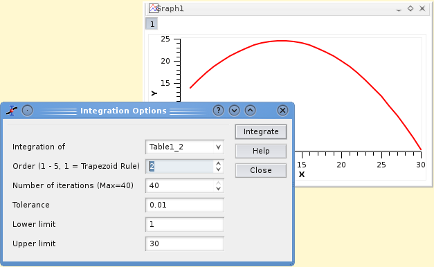
Opens the integration dialog, allowing to choose the curve to integrate and the integration method. This command can't be used to obtain a cumulative curve from a selected curve, it can only compute the integral of the data between two limits.
The first field is the curve that will be integrated. The second one is the order of the integration: the order 1 corresponds to the trapezoid rule, i.e. the curve is aproximated by a straight line between 2 successive points. If you choose the order 2, three successive points are used and a second order polynome is used to approximate the curve. etc. If you have a large amount of points in your curve, the order 1 is enough.
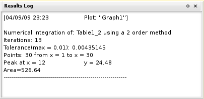
The result of the integration will be given in the Results Log.
- Smooth
-
These commands will generate a new curve by dooing a smoothing ofthe selected curve.
- Smooth→Savitsky-Golay
-
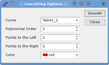
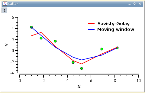
This command performs a smoothing of the selected curve with the Savitzky-Golay method. The formula used to smooth the curve defined by the points yi=f(xi) is:
The fi values are computed by fitting the data points to a polynome, they depend on the number of points used for the smoothing of the curve and the order of the polynome. Compared to the moving window average method, the advantage of this smoothing method is that the values of extrema are not truncated. The dialog allows to specify the curve which will be smoothed, the value of the order of the polynome, the number of data points used for the polynomial fit before and after each point and the color used to draw the smoothed curved. A new table will be created to store the data points xi, zi.
- Smooth→Moving Window Average
-
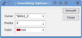
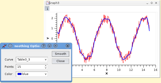
This command performs a smoothing of the selected curve with the moving window average method. The formula used to smooth the curve defined by the points yi=f(xi) is:
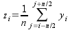
The greater the number of points n, the smoother the resulting curve zi=f(xi) is. The dialog allows to specify the curve which will be smoothed, the value of n and the color used to draw the smoothed curve. A new table will be created to store the data points xi, zi.
Depending on the number of data points and on the variation of the Y values, smoothing can give very different results.
- Smooth→Moving Window Average
-
This command allow a smoothing based on FFT filtering of data. It can be used when you have noisy curves with a large number of data.
- FFT Filter
-
- FFT Filter→Low Pass
-
This command allows to filter the high frequencies of a signal. See the filtering section for more details. A dialog box will be opened in which you can select the curve to filter and the cut-off frequency of the filter.
This command creates a new table with the filtered data, and a new curve will be added on the current plot. See the section called “Filtering of data curves” of the Chapter 3, Analysis of data and curves for details.
- FFT Filter→High Pass
-
This command allows to filter the low frequencies of a signal. See the filtering section for more details. A dialog box will be opened in which you can select the curve to filter and the cut-off frequency of the filter.
This command creates a new table with the filtered data, and a new curve will be added on the current plot. See the section called “Filtering of data curves” of the Chapter 3, Analysis of data and curves for details.
- FFT Filter→Band Pass
-
This command allows to filter the low and high frequencies of a signal. See the filtering section for more details. A dialog box will be opened in which you can select the curve to filter and the cut-off frequency of the filter.
This command creates a new table with the filtered data, and a new curve will be added on the current plot. See the section called “Filtering of data curves” of the Chapter 3, Analysis of data and curves for details.
- FFT Filter→Block Band
-
This command allows to keep the low and high frequencies of a signal. See the filtering section for more details. A dialog box will be opened in which you can select the curve to filter and the cut-off frequency of the filter.
This command creates a new table with the filtered data, and a new curve will be added on the current plot. See the section called “Filtering of data curves” of the Chapter 3, Analysis of data and curves for details.
- Interpolate
-
Performs an interpolation. The curve must have enough data points to compute the interpolated points, if not a warning message will be prompted out.
The methods available to perform the interpolation are Linear (the curve must contain at least 3 points), Cubic Spline (the curve you analyse must contain at least 4 points, if not a warning message will be prompted out, Non-rounded Akima spline (the curve you analyse must contain at least 5 points). See the the section called “Interpolation” of the Chapter 3, Analysis of data and curves for a comparison of the differents methods.
This command creates a new curve on the current plot, and a new table.
- FFT
Performs a forward or inverse FFT transform of the selected curve. The inverse FFT transform of a forward transform will result in a data set identical to that used for the forward transform.
- Quick Fit
-
- Quick Fit→Fit Linear
Performs a linear fit of the selected curve. The results will be given in the Log panel
- Quick Fit→Fit Polynomial
Opens the Polynomial Fit dialog, allowing you to choose the curve to fit, the order of the polynomial function to use, the number of points of the resulting curve and the abscissae limits for the fit.
- Quick Fit→Fit Exponential Decay
-
- Quick Fit→Fit Exponential Decay→First Order
Opens the Exponential Fit dialog, allowing you to choose the curve to fit and the initial guesses for the fit parameters.
- Quick Fit→Fit Exponential Decay→Second Order
Opens a dialog, allowing you to choose the curve to fit and the initial guesses for the fit parameters.
- Quick Fit→Fit Exponential Decay→Third Order
Opens a dialog, allowing you to choose the curve to fit and the initial guesses for the fit parameters.
- Quick Fit→Fit Exponential Growth
Performs an exponential growth fit of the selected curve.
- Quick Fit→Fit Lorentzian
Performs a lorentzian fit of the selected curve. It can be used to obtain a correlation equation of a bell shaped data set (see the section called “Fitting to a Lorentz function” for details).
- Quick Fit→Fit Gaussian
Performs a gaussian fit of the selected curve.It can be used to obtain a correlation equation of a bell shaped data set (see the section called “Fitting to a Gauss function” for details).
- Quick Fit→Fit Bolzmann (Sigmoïdal)
Performs a fit to a bolzmann function of the selected curve. It can be used to obtain a correlation equation of a S shaped data set. (see the section called “Fitting to a Bolzmann function” for details).
- Quick Fit→Fit Multipeak
-
- Quick Fit→Fit Multipeak→Gaussian
Performs a fit to a sum of N gaussian functions of the selected curve. (see the section called “Multi-Peaks fitting” for details).
- Quick Fit→Fit Multipeak→Lorentzian
Performs a fit to a sum of N lorentz functions of the selected curve. (see the section called “Multi-Peaks fitting” for details).
- Fit Wizard (CTRL+Y)
Performs a fit of the selected curve. This opens the general dialog for the fitting of curves. See the the section called “Non Linear Curve Fit” for a tutorial on this command. Some default parameters can be modified with the Preferences command, see the the section called “Changing default parameters for fitting” for details