Chapter 3. Analysis of data and curves

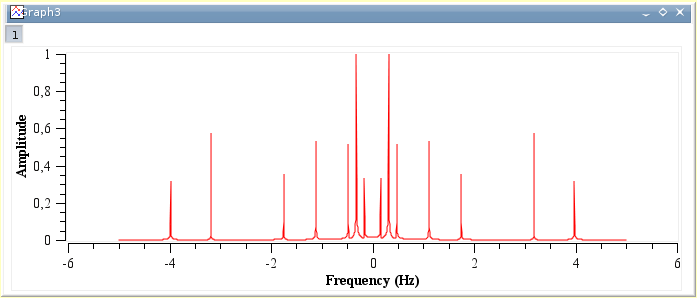
This function can be accessed by the FFT command of the Analysis-tables menu when a table is selected, or Analysis-plots menu when a plot is selected. The Fourier transform decomposes a signal in its elementary components by assuming that the signal x(t) can be describe as a sum:

in which ω_n are the frequencies, a_n are the amplitudes of each frequency and ψ_n are the phase corresponding frequency. SciDAVis will compute these parameters and build a new plot of the amplitude as a function of the frequency. FFT can be performed on a curve to extract the characteristic frequencies.

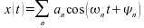
Let's assume you have the signal presented in the next figure. You can select the FFT command of the Analysis-plots menu to open the FFT dialog box.

If the Normalize Amplitude check box is on, the amplitude curve is normalized to 1. If the Shift Results check box is on, the frequencies are shifted in order to obtain a centered x-scale. By default, the Sampling Interval corresponds to the interval between X-values. Giving a smaller value makes no sense, but you can increase this value in order to sample less values.

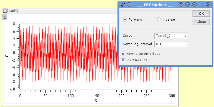
SciDAVis will create a new plot window with the FFT amplitude curve, and a new table which contains the real part, the imaginary part, the amplitude, and the angle of the FFT. In this example, the amplitude curve has been normalized, and the frequencies have been shifted to obtain a centered x-scale.

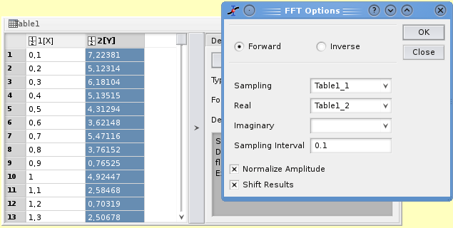
In the case of a table, you must select the sampling column (X-values) and one columns (for real numbers) or two columns (for complex numbers) for Y-values.