Fitting can be done in two ways:
A general Fit Wizard which allows to use complex functions and to adjust the fitting parameters.
A set of simplified fitting dialog boxes for most used functions like exponential growth or decay, etc.
This function can be accessed by the Fit Wizard command of the Analysis-plots menu when a plot is selected, or the Analysis-tables menu when aa table window is selected. In the latter case, this command first creates a new plot window using the list of selected columns in the table.
This Command is used to fit discrete data points with a mathematical function. The fitting is done by minimizing the least square difference between the data points and the Y values of the function.
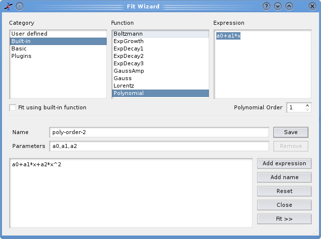
The top of the dialog box is used to choose a function among the one which are already define. Four types of functions are available: the user defined functions which have been saved, the classical functions proposed by SciDAVis in the analysis menu, the simple elementary built-in functions, and external functions via pluggins.
To choose one of these functions, you just have to select it and to click on the checkbox under the selector.
If you want to define your own function, you can use the bottom half of the dialog box. You can write you own mathematical expression or add expressions obtained with the function selector. Then you need to define the parameters which have to be fitted in a comma separated list.
The second step is to define the parameters for the fit. You have to give initial guess for the fitting parameters.
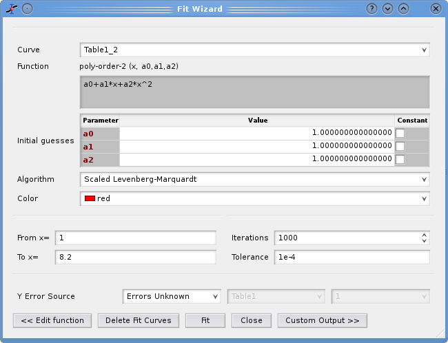
In this second tab you can also choose a weighting method for your fit (the default is No weighting). The available weighting methods are:
Instrumental: the values of the associated error bars are used as weighting coefficients. You must add Y-error bars to the analyzed curve before performing the fit.
Statistical: the weighting coefficients are calculated as the square-roots of each data point in the fitted curve.
Arbitrary Dataset: you have the possibility to set the weighting coefficients using an arbitrary data set. The column used for the weighting must have a number of rows equal to the number of points in the fitted curve.
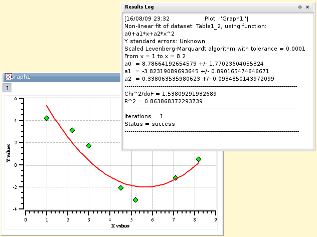
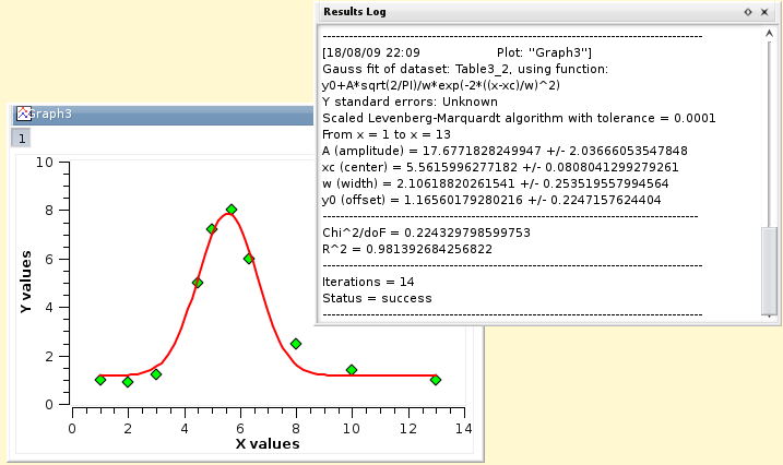
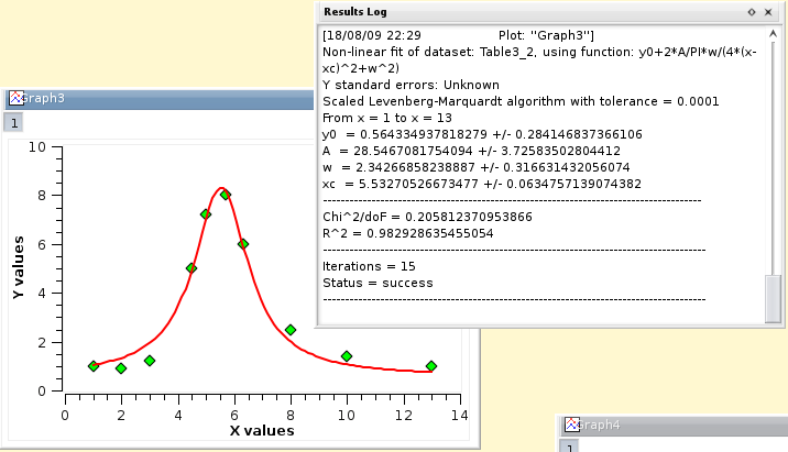
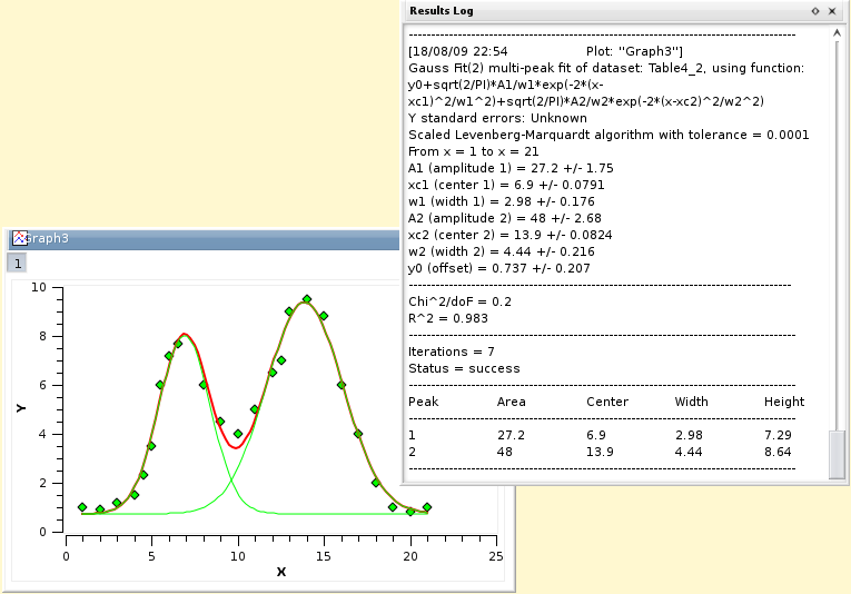
After the fit, the log window is opened to show the results of the fitting process.
Depending on the settings in the Custom Output tab, a function curve (option Uniform X Function) or a new table (if you choose the option Same X as Fitting Data) will be created for each fit. The new table includes all the X and Y values used to compute and to plot the fitted function and is hidden by default, but it can be found and viewed with the project explorer.
Figure 3.12. The results of the Fit Wizard.
The results are shown in the log window, the curve is plotted in the active window, and a table is created to store the fit.
SciDAVis include quick access to the most usefull functions for fitting. Beware that when you use these commands, SciDAVis uses default values as initial guesses for the parameters. Therefore, the convergence may be difficult or even impossible if these initial values are too far from the final values. In this case, you can use the Fit Wizard command or the Fit Wizard command, select the function in the built-in set and give good initial values for parameters.
This command is used to fit a curve which has a linear shape. The results will be given in the Log panel.
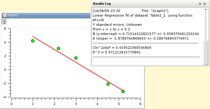
This command is used to fit a curve which has a linear shape. The results will be given in the Log panel
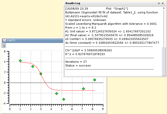
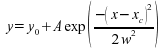
This command is used to fit a curve which has a sigmoidal shape. The function used is:
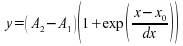
in which A2 is the high Y limit, A1 is the low Y limit, x0 is the inflexion point and dx is the width.
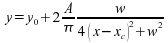
This kind of fitting allows to fit your data points to a sum of N Gaussian or Lorentzian functions. The first step is to specify the number of peaks. Then you must define the position of each peak on the curve. This is done by selecting one data point on the plot, then validate your choice for each peak with the ENTER key.
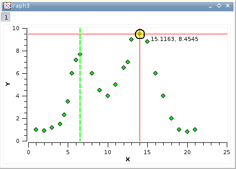
Then, the fitting is done in the same way as for the other quick-fit commands. For the position of the data points used for the selection of the position of the peaks are just initial guesses for the fitting.
As for the other quick-fit commands, if you want to fit with a sum of more complex curves (e.g. a combination of lorentzian and gaussian functions), use the Fit Wizard.
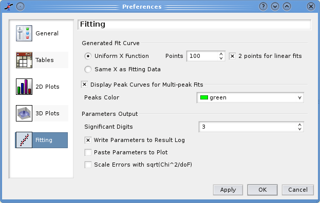
This dialog can be accessed by the Preferences command of the Edit menu. It allows to modify the way the fitted curves are drawn on the plots and some options for the presentation of the fitted values. If you want to modify some parameters related to the fitting itself, like the tolerance, you have to do it in the Fit Wizard.