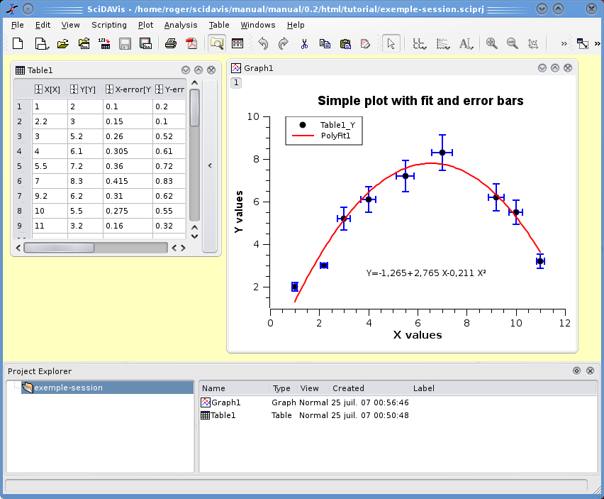
Several plots and all the data related to these plots can be save in a project file, the project is therefore the main container of SciDAVis. The following screenshot gives an example of a typical session. This example shows the log panel at the top of the workspace, the project explorer at the bottom, a table and a plot window are shown while other are docked or hidden.
There are numerous commands available in SciDAVis depending on the element which is selected. Therefore, the main menu bar changes when you select a particular element of the project. Moreover, you can access to the set of commands relevant of an element by activating the context menu with the right button of the mouse.
In a project, the objects which can be used are:
- Tables
-
A table is a spreadsheet which can be used to store the datas you are entering. It can also be used to do some calculations and statistical analysis of datas. In each table, columns can be labelled as X-values or Y-values for 2D-plotting, or Z-values if you plan to build a 3D-plot. In addition, columns can be labelled as errors on X or on Y values (see Set Column as command).
A table can be created by the New→New Table command. Then there are several ways to fill the table with your data. If you want to read a table from an ASCII file, you can import the data from the file to a table with the Import Ascii command. You can also enter each value from the keyboard, or copy and paste from another spreadsheet software. The last way to enter your data is to fill the table with the results of a mathematical function (Assign Formula command from the Table menu)
- Matrix
-
A matrix is a special table which is used to store the data points for surface 3D plots. It contains Z-values and doesn't include any column or row which could be designed as X-values or Y-values. Nevertheless, you can specify the X-values and the Y-values with the Set Coordinates command command from the Matrix menu.
A matrix can be created by the New→New Matrix command. If you want to read a matrix from an ASCII file, you can import the data of the file to a table with the Import Ascii command and then convert this table to a matrix with the Convert to Matrix command. In the same way as for tables, you can also fill matrix with the results of a function z=f(i,j) in which i and j are row and column numbers, or z=f(x,y). (see Assign Formula command from the Matrix menu)
- A Graph
-
A graph can contain one or several plots. Each of these plots is contained in a different layer, these layers can be arranged in many ways to build matrix of plots.
A new layer can be added to an existing graph with the Add Layer command from the Graph menu. you can also remove an existing layer with the Remove Layer command, but if you remove a layer, the plot will be deleted. You can also copy a layer from one graph to another, or copy an existing graph into another, the window will be added as a new layer (see the section on Multilayer Plots for more details).
Plots can be created in several ways. You can select data in tables or matrix and build a plot, or create new plots from functions of one or two variables (see sections 2D plots and 3D plots).
- A Note
This window is a text container which can simply be used to insert comments into a project. This object is nevertheless far more powerfull than that: it can be used as a calculator, for executing single commands and for writing scripts (see the Scripting section for more details).
- The Log Window
-
This window is used to store the results of all the calculations which have been done. If this window is not visible, you can find it with the Project Explorer or with the Results Log command.
The text in the log window is also saved in the project file, so that when you load a previously saved project, the results-log panel is re-filled with the results of the calculations.
- The Project Explorer
-
This window is used to list all the windows contained in a projet. The Project Explorer is opened by the Project Explorer command, and gives a quick access to all elements of a project, hidden or visibles. It can be used to do some operations on the windows related to these items such as hidding a window, renaming windows, etc.
A project file can include several independant projects. In this case, the containers of each project are stored in different folders.
The table is the main part of SciDAVis when working with data. For controlling and converting data the spreadsheet contains a highly customizable table: all colors and font preferences can be set using the Preferences command of the Edit menu. You can resize a table in terms of rows and columns using the Dimensions command command of the Table menu. On the left side of the table, the button can be used to develop the properties tags. This allows to customize the main parameters of the table.
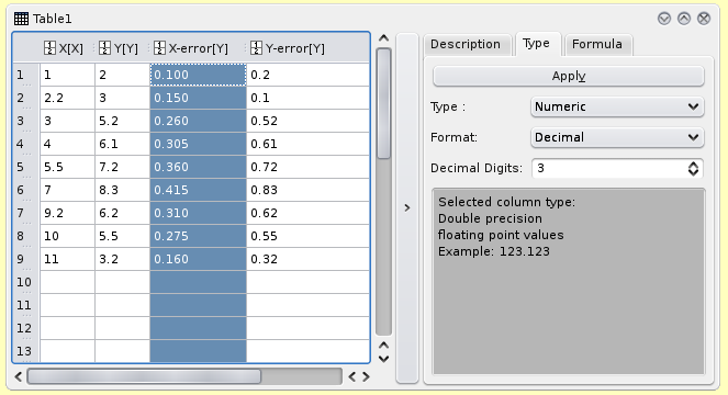
In a spreadsheet, columns can have the following flags: X, Y, Z, X-error, Y-error or can be simple columns without any special flag. The X columns are abscissae columns while the Y columns are ordinates columns used when creating a 2D plot from data. The X-error and Y-error columns can be used in order to add error bars to 2D plots. These flags can be changed using the Set Column as command.
The tag which is selected in figure 1.2 is used to assign a type to columns: numeric, text, date or time. The format used to display the data can then be chosen, the format in tables is not used for plots (use the Axes command to define display format for axes labels).
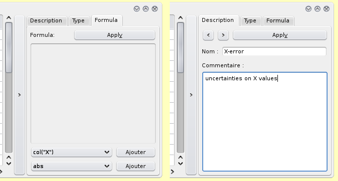
Every column of the table has a label, this can be defined in the description tag (figure 1.3). This label will be used by default in plots for curve selection and legend display. You can use complex labels with spaces and special characters like "Vol (cc/g)" if needed. This command can also be reached by the Edit Column Description command of the Table menu.
The last tag of the properties dialog correspond to the command Assign Formula command of the Table menu (figure 1.3). It is used to fill the column with the result of a mathematic expression. Refer to the Assign Formula command for more details.
You can select all the columns of the spreadsheet (Ctrl+A) or only some of them by clicking on the column label while keeping the Ctrl key pressed, or by moving the mouse over the column label. This also allows you to deselect columns.
On the selected columns you can perform various operations:
Fill with data. You can insert the row numbers (Fill Selection With→Row Numbers command), random numbers (Fill Selection With→Random Values command), or the result of a function (Assign Formula command);
normalize columns with the Normalize Columns command of the context menu;
sort columns with the Sort Table command of the Table menu or with the sort column command of the context menu;
compute statistical data on columns and rows with the Statistics on Columns command and Statistics on Rows command of the Analysis-tables menu;
build a plot from selected columns with the plot command of the context menu or with the commands of the Plot menu.
All these functions can be reached by right clicking when a column is selected. Most of them can also be reached by using the Table menu.
You can cut, copy and paste data between spreadsheets or between a spreadsheet and another application (Excel, Gnumeric, OpenOffice Calc, etc).
You can import single or multiple ASCII files using the Import Ascii command from the File menu. This will create one or more new tables. You can also export the data from the spreadsheet to a text file using the Export Ascii command.
The matrix is a special table which is used for data which depends on two variables. This special table is used to store data for 3D-plots. The difference between a table and a matrix is that there is that columns are assigned to the abscissae x while rows define abscissae y.
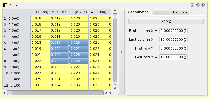
The defaut size of a matrix is 32x32 cells. You can modify this size with the Dimensions command. Column and row numbers are named i and j respectively, ranging from 1 to the size of the matrix. You can specify an X-scale and an Y-scale with the Set Coordinates command, this define values of x and y for columns and rows (figure 1.4).
The values which are stored in a matrix can be obtained from a function of the form z=f(i,j) or z=f(x,y) with the Assign Formula command. They can also be read from a file with the Import Ascii command which allows to read a file in a table, then the table can be converted to a matrix with the Convert to Matrix command of the Matrix menu.
As in the case of tables, a property tag can be shown or hidden by clicking on the vertical button on the right.
Through the Matrix menu, several operations can be done on a matrix like transposition (Transpose command), mirroring (Mirror Horizontally command and Mirror Vertically command), inversion (Invert command), computation of the determinant (Determinant command). The data of a matrix can then be used to build a 3D plot with the commands present in the plot3d menu and in 3D surface toolbar.
The plot window is the one in which the graphic is plotted. The main container of the plot window is the layer. You can have several layers in a plot, which may be arranged as you want. Each layer can contain a plot, or another item like a label.
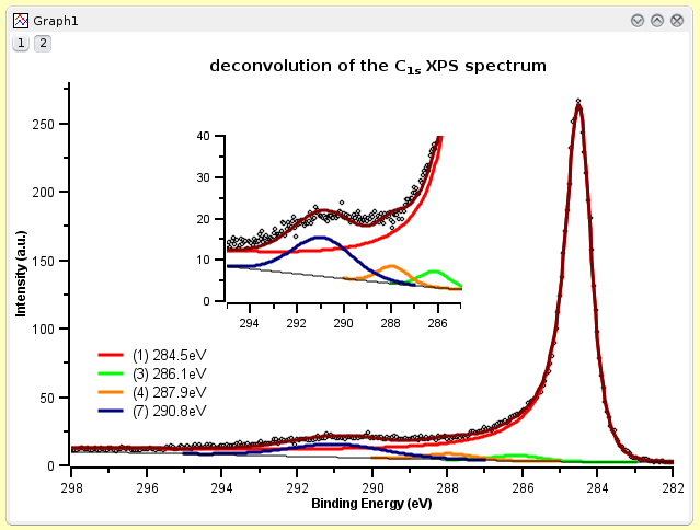
Each new plot can be inserted in a new layer of this plot window, it has its own geometry and graphic properties (background color, frame, etc). The figure 1.5 shows a graph with two layers which have different geometries. Inside a layer, the area in which the curves are plotted is the canvas.
Each layer can be activated by clicking on the corresponding gray button  in the top-left corner of the window. The elements which can be accessed by a double click in a layer are:
the graph itself: this will open the Plot details dialog box. You can then change the way the curves are plotted.
The axes or the axes labels: this will open the General Plot Options Dialog. It is used to customize the axes, the numbers and labels of the axes, and the grid.
Any other text item: this will open the Text Dialog which allows to customize the font of the label and the frame in which it is drawn.
All these functions can be reached through the Format menu.
A note can simply be used to insert text (comments, notes, etc) into a project, but is really far more powerfull than that. It can be used as a calculator, for executing single commands and for writing scripts.
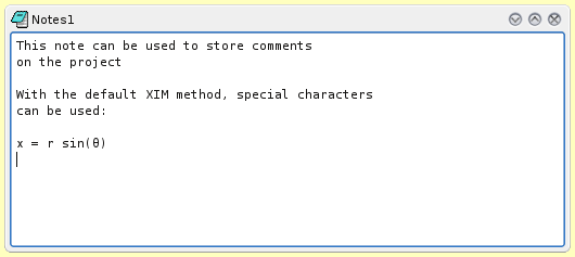
You can also change the text input method. Simple Composing Input Method is the standard method to enter text in QT applications. Xim is the X input method, it is the legacy system of the X window environment to support localized text input. The default choice is the second one, it allows to enter special characters and accents from your localised environment.
The second use of notes is calculator. The evaluation of mathematical expressions and execution of code is done via a note's context menu, the Scripting menu or the convenient keyboard shortcuts. In figure 1.7, it is shown that you just need to place the cursor on an expression and use the Ctrl-Return command to evaluate the expression.
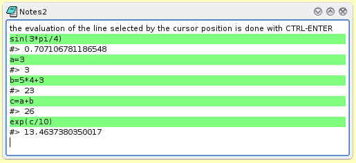
you can define variables and refer to them to build complex expressions, but you must evaluate each line with the Ctrl-Return command to fill the variable with its value. All variable are private to the note in which it is defined, and you can't refer to it in another note. With a right click, you access to the context menu which contains the list of all available mathematical functions.
For information on expression syntax, supported mathematical functions and how to write scripts, see the scripting section.
This window keeps a history of all analysis which have been done in the project. This panel contains the results of all the correlations, fittings, etc. It can be shown or hidden with the Results Log command of the View menu.
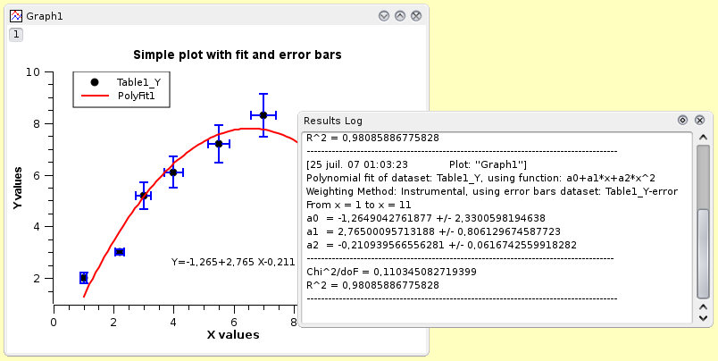
You can clear the content of the log window with the command Clear Log Information command of the Edit menu. If you load a project for which some analysis has been done, the computations will be done again and the log window will be filled with the results.
The project explorer can be opened/closed using the Project Explorer command from the View menu or by clicking on the ![]() in the file toolbar.
in the file toolbar.
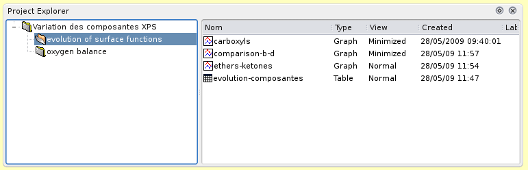
It gives an overview of the structure of a project and allows the user to perform various operations on the windows (tables and plots) in the workspace: hiding, minimazing, closing, renaming, printing, etc... These functions can be reached via the context menu, by right-clicking on an item in the explorer.
By double-clicking on an item, the corresponding window is shown maximized in the workspace, even if it was hidden before.
You can organize the differents objects in folders. When selecting a folder, the default policy is that only the objects contained in it will be showed in the workspace window. You can also display all the objects in the subfolders if you change this policy with the "View Windows" command to "Windows in Active Folder and Subfolders".