3D plot are generated from data defined as Z=f(X,Y). As for 2D plots, there are two ways to obtain a 3D plot depending on the way the (X,Y,Z) values are defined:
-
You can have your Z values in a matrix. SciDAVis will consider that all the data present in the matrix are Z values, and the X and Y values can be defined as a linear function of the columns and rows numbers.
The data in the matrix can be entered in several ways:
one by one from the keyboard,
by reading an ascii file in a table and converting the table into a matrix,
by setting the values with a function.
If you want to plot a function, you don't need a matrix. You can use directly the New→New 3D Surface Plot command.
There are several kinds of 3D plots which can be selected, see the plot3d menu section of the reference chapter for a list of the availables plots.
The 3D plots use OpenGL so you can easily rotate, scale and shift them with the mouse. Via the 3D plot settings dialog or via the Surface 3D Toolbar you can change all the predefined settings of a three dimensional plot: grids, scales, axes, title, legend and colors for the different elements.
There are several types of plots which can be built from a matrix. They are presented in the plot3d menu
This is the simplest way to obtain a 3d plot. It is done with the New→New 3D Surface Plot command from the File menu or directly with the CTRL+ALT+Z. This will open the following dialog box:
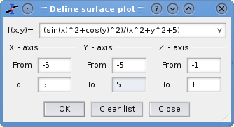
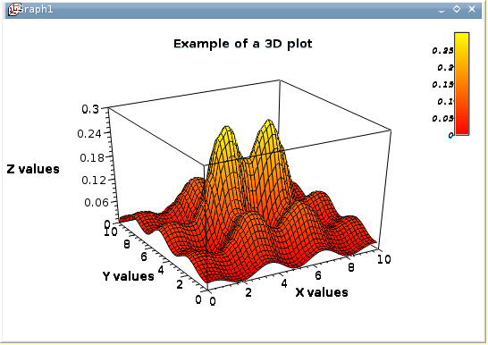
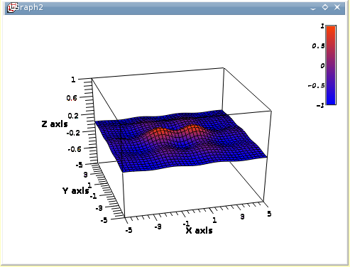
You can enter the function z=f(x,y) and the ranges for X, Y and Z. Then SciDAVis will create a default 3d plot:
You can then customize this plot by opening the Surface plot options dialog. You can modify the axis ranges and parameters, add a title, change the colors of the different items, and modify the aspect ratio of the plot. In addition, you can use the different commands of the 3D surface toolbar to add grids on the walls or to modify the style of the plot. After some modifications, you can obtain the plot presented above.
If you want to modify the function itself, you can use the surface... command which can be activated from the context menu with a right click on the 3D plot. This will re-open the define surface function dialog box.
The 3D plotting system uses openGL, therefore these plots can be manipulated with the mouse:
by clicking on the left button and moving the mouse, you can change the viewpoint of the plot. You can come back to the default viewpoint by clicking on the
 icon of the 3D surface toolbar.
The ??? can be used to zoom or unzoom the plot. You can come back to the default zoom value by clicking on the
 icon of the 3D surface toolbar.
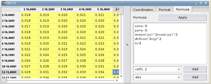
The second way to obtain a 3D plot is to use a matrix. Therefore, the first step is to fill the matrix. This can be done by defining a function.
The New→New Matrix command create a default empty matrix with 32x32 cells. Then use the Dimensions command from the Matrix menu to modify the number of rows and columns of the matrix. The Set Coordinates command can then be used to define the X and Y ranges.
Then use the Assign Formula command to fill the cells with numbers. The ranges of X and Y defined in the previous step are not known by this dialog box, then the function is defined with the row and column numbers (i and j) as entry parameters.
The other way to obtain a matrix is to import an ASCII file into a table with the Import Ascii command from the File menu. The table can then be transformed in a matrix with the command Convert to Matrix command from the Table menu.
You can then use this matrix to build a 3D plot with one of the command of the Plot menu.
A dialog with five tab is activated by double clicking on a contour curve (or on the plotting area) of a 3D plot. It can also be accessed by the commands of the Format menu.
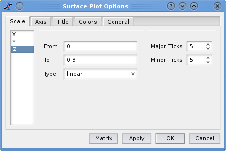
The first group of settings Scales is used to define the scales of the three axis. It works in the same way as scaling of 2D plots.
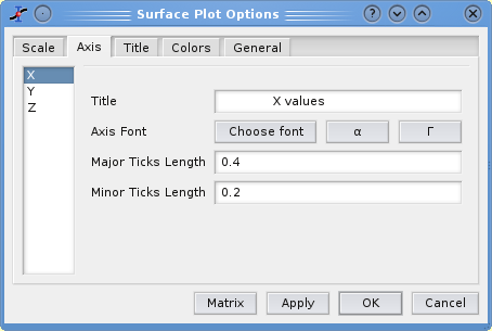
The second tab Axis is used to define the labels of the three axis. You can also customize the size of the ticks, beware that this size is given in real units. Therefore, it should be chosen in relation to the axis ranges: for example, if you put a length of 1 for the ticks of the X-axis, the length will correspond to a unit of 1 from the Y axis. In the same way, Y and Z ticks are computed in reference to X range.
The third tab Title is used to modify the title of the plot. Compared to conventional label dialog box of SciDAVis, it exhibits some limitations related to the 3D drawing system (no subscripts, superscript, no bold or italic characters). See the Title command for more details.
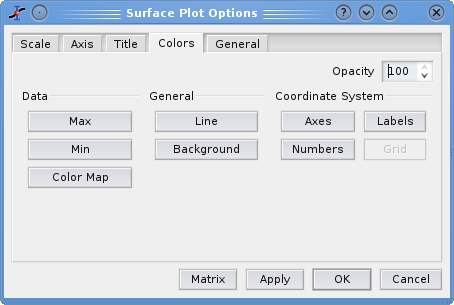
The fourth tab Colors is used to modify the color of the different elements. For General and Coordinate System elements, it is a conventional choosing color dialog box. You can also customize the colormap used to draw the data. See the next section for more details on color maps.
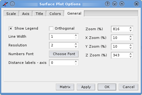
The last tab General is used to modify some global parameters of the plots. The orthogonal check box allows to change the 3D view from conventional perspective to orthogonal view. It correspond to the ![]() icon of the 3D surface toolbar. The parameter resolution is 1 by default, it indicates that all data points are used to draw the contour curves. If the line network is too dense, you can increase this parameter: with a value of 2 only 1 value over 2 will be used.
icon of the 3D surface toolbar. The parameter resolution is 1 by default, it indicates that all data points are used to draw the contour curves. If the line network is too dense, you can increase this parameter: with a value of 2 only 1 value over 2 will be used.
By default, the plot use the same graphic scales for the three axes. If the ranges are very different, you can adjust the size of the plot by changing the zoom over the different axes. In the example presented above, X and Y ranges are 10 while Z range is 0.2, then a zoom of 3000% should be used for Z axis if the zooms on X and Y are kept at 100%. You can also use the ![]() icon of the 3D surface toolbar to adjust automatically these zoom values.
icon of the 3D surface toolbar to adjust automatically these zoom values.
The two colors (data min and data max) defines the color scheme which is used to show the Z-values. They are the colors used for the minimum value of Z (Zmin) and the maximum value of Z (Zmax). We can define the colors by their Red, Green and Blue parameters: [R,G,B]. Then, a value Z will be represented by a color defined as a linear interpolation:
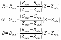
The default colors for Zmin and Zmax are respectively blue ( [R,G,B] = [0,0,255] ) and red ( [R,G,B] = [255,0,0] ). This lead to the following color scheme:

Another classical color scheme can be built with Zmin = [160,32,32] and Zmax = [255,255,0] (yellow). It leads to:

Another way to define colors is to read a colormap from a file. The format of the file is simple: each line defines a color by red, green and blue values as integers between 0 and 255. The numbers should be separated by spaces. You can find several examples of colormaps on the QwtPlot3D web site.
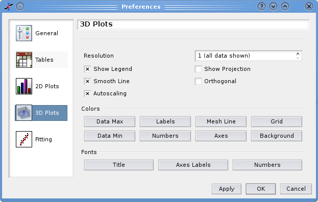
Most of the parameters presented in the previous section can be set by default with the Preferences command of the Edit menu.